请欣赏一下Mathematica绘制的漂亮的函数图~ヾ(^▽^)
1 | Plot[{(1 + 1/n)^n, Evaluate[Limit[(1 + 1/n)^n, n -> Infinity]]}, {n, 0, 100}, PlotLegends -> "Expressions"] |
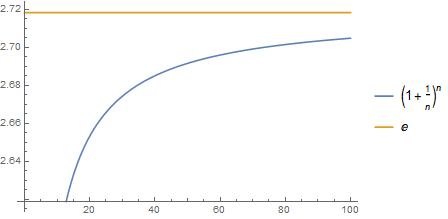
形象地展示了 $\lim\limits_{n \rightarrow \infty}{(1+\frac{1}{n})^n}=e$ 的过程。
1 | Plot[{n^(1/n), Evaluate[Limit[n^(1/n), n -> Infinity]]}, {n, 0, 1000}, PlotLegends -> "Expressions"] |
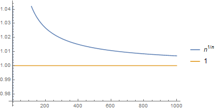
形象地展示了 $\lim\limits_{n \rightarrow \infty}{n^{\frac{1}{n}}}=1$ 的过程。
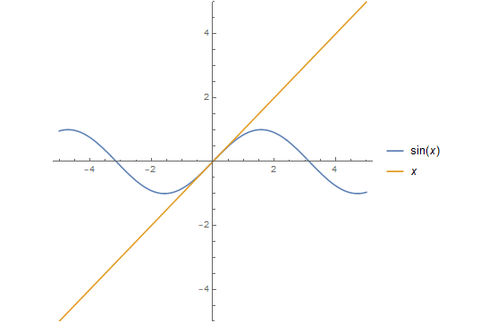
1 | Plot[{Sin[x]/x, Evaluate[Limit[Sin[x]/x, x -> 0]]}, {x, -4*Pi, 4*Pi}, PlotLegends -> "Expressions"] |
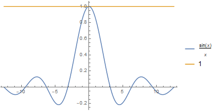
形象地展示了 $\lim\limits_{x \rightarrow 0}{\frac{sin(x)}{x}}=1$ 的过程。
1 | Plot[{x*Sin[1/x], x, -x}, {x, -0.1, 0.1}, PlotRange -> 0.1, AspectRatio -> 1, Filling -> Axis] |
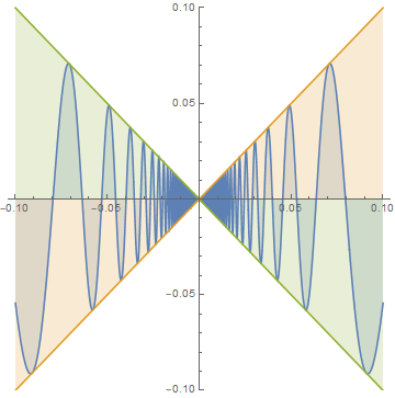
形象地展示了 $\lim\limits_{x \rightarrow 0}{(x\ sin(\frac{1}{x}))}=0$ 的过程。(⊙o⊙)
1 | t = Table[Plot[f[x], {x, -2*Pi, 2*Pi}, PlotRange -> 2*Pi, AspectRatio -> 1, ExclusionsStyle -> Dashed, PlotLabel -> f], {f, {Sin, Cos, Tan, Cot, Sec, Csc}}]; |
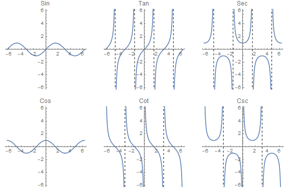
上篇文章中的例子,加了渐近线和标签,坐标轴等比例化,再将列表组合成一张图,好看一些。
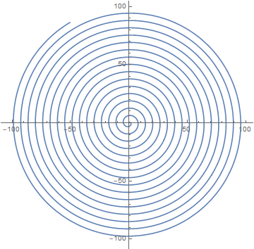
1 | ParametricPlot[{u*Sin[u], u*Cos[u]}, {u, 0, 100}] |
添加一点选项:
1 | ParametricPlot[{u*Sin[u], u*Cos[u]}, {u, 0, 100}, PlotPoints -> 125, Axes -> False, MaxRecursion -> 0, ColorFunction -> "Rainbow"] |
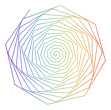
像一朵花。
1 | Plot3D[x^2 - y^2, {x, -1, 1}, {y, -1, 1}, BoxRatios -> {1, 1, 1}] |
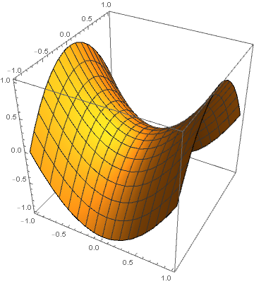
画一个马鞍面。
1 | ParametricPlot3D[{Sin[t], Cos[t], t}, {t, 0, 100}, BoxRatios -> {1, 1, 1}, ColorFunction -> "Rainbow"] |
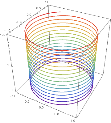
画一个彩色弹簧。
1 | PolarPlot[Sin[6*t] + 0.1*RandomReal[], {t, 0, 2*Pi}, ColorFunction -> Hue, Axes -> False] |

1 | f = Sin[Range[0, 12*Pi, 0.1]]; |

漂亮的花。
1 | ListPointPlot3D[Table[{r*Cos[t], r*Sin[t], Sinc[r]}, {r, 0, 3*Pi, 0.1}, {t, 0, 2*Pi, 0.1}], Boxed -> False, Axes -> False] |
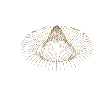
草帽~
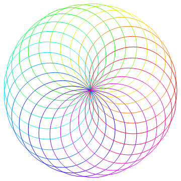
1 | Graphics[Table[{Hue[t/25], Circle[{Cos[(2*Pi*t)/25], Sin[(2*Pi*t)/25]}]}, {t, 25}]] |
1 | Graphics3D[{Red, Ball[{0, 0, 2}], Blue, Cuboid[{-1, -1, -1}, {1, 1, 1}]}, Boxed -> False] |
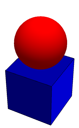
还可以练素描。
1 | RegionPlot3D[x^2 + z^2 <= 1 && y^2 + z^2 <= 1, {x, -1, 1}, {y, -1, 1}, {z, -1, 1}, PlotPoints -> 40, Mesh -> None, Boxed -> False] |
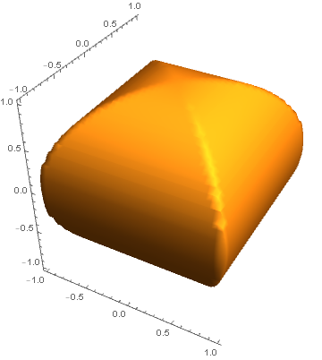
牟合方盖。
1 | Animate[Plot[Evaluate[{Sin[x], Normal[Series[Sin[x], {x, 0, n}]]}], {x, -5, 5}, PlotRange -> 5, AspectRatio -> 1, PlotLegends -> "Expressions"], {n, 1, 10, 2}] |
泰勒级数的可视化。
1 | Animate[Plot[(x^n & )[x, n], {x, -10, 10}, PlotRange -> 10, AspectRatio -> 1], {n, -5, 5, 0.1}] |
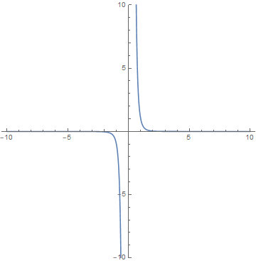
幂函数的可视化。
1 | Animate[Plot3D[Sin[Sqrt[x^2 + y^2] + 2*Pi*t], {x, -8*Pi, 8*Pi}, {y, -8*Pi, 8*Pi}, PlotRange -> 10, PlotPoints -> 50, AspectRatio -> 1, Boxed -> False, Mesh -> None, Axes -> False], {t, 0, 2}] |
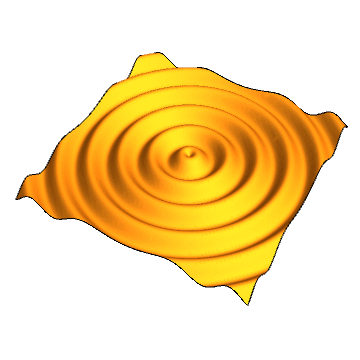
水面波纹效果~
1 | MandelbrotSetPlot[] |
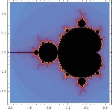
Mathematica内置了许多函数图,曼德勃罗集合图是其中之一。这被称为“上帝的指纹”。